Researching for two days is not really that long. It is an interesting topic though for sure. @D Stanley's answer is spot on. I just like to add (likely TL;DR) details to suit the comment
Now, someone could maybe come up with a more accurate representation of that probability distribution, but the calculus might not be as neat as it is with a "normal" distribution.
There is no general IV for an option. Quoting from Just What You Need To Know About Variance Swaps - JP Morgan Equity Derivatives
For each strike and maturity there is a different implied volatility
which can be interpreted as the market’s expectation of future
volatility between today and the maturity date in the scenario implied
by the strike. For instance, out-of-the money puts are natural hedges
against a market dislocation (such as caused by the 9/11 attacks on
the World Trade Center) which entail a spike in volatility; the
implied volatility of out-of-the money puts is thus higher than
in-the-money puts.
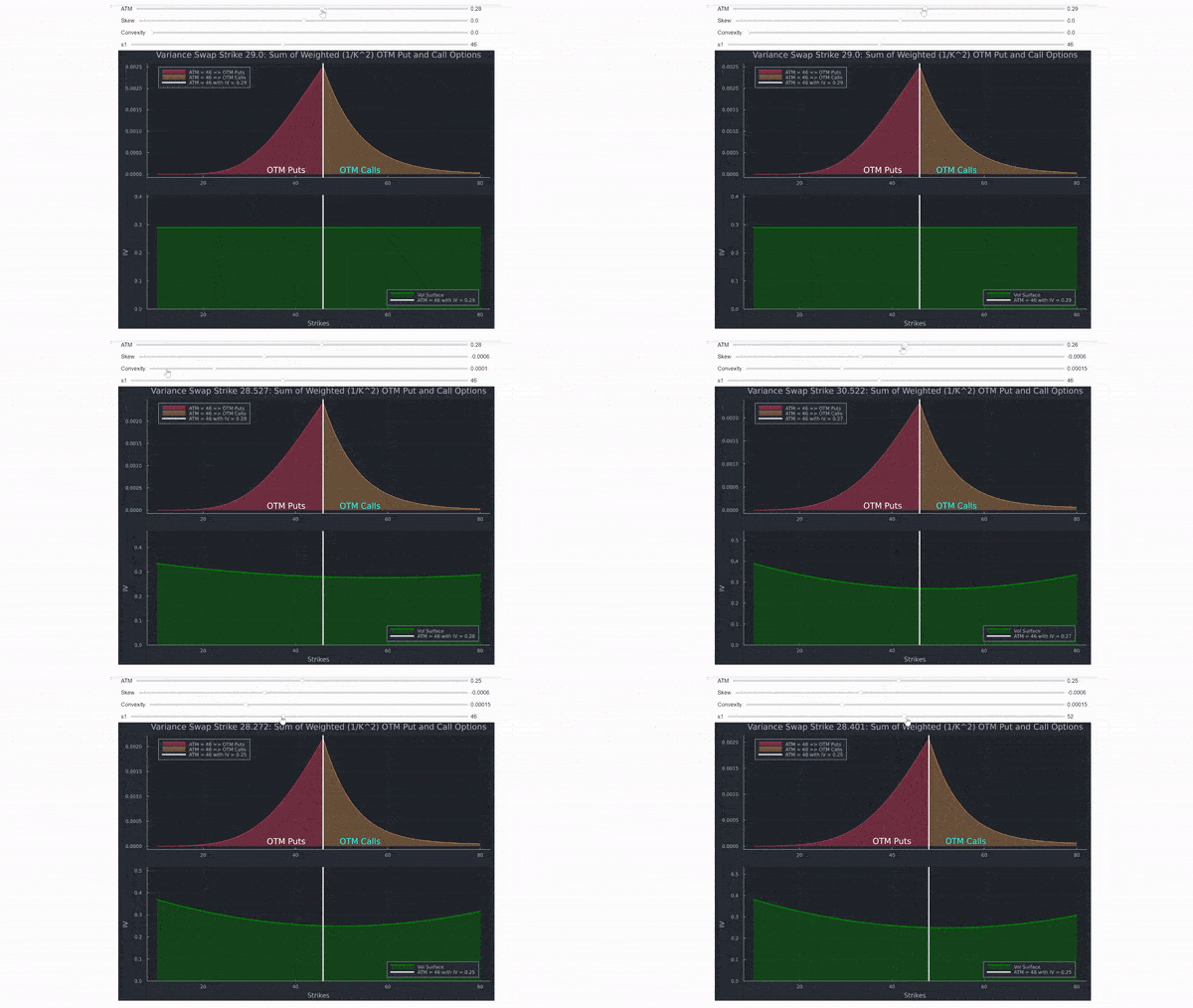
What most people refer to if they look at a single vol is the ATM volatility. Sometimes also a VIX like measure. The VIX is the square root of the variance swap strike, computed via SPX options that are listed for trading on the Cboe. This answer explains what this computation looks like. The gif from the answer looks like this:

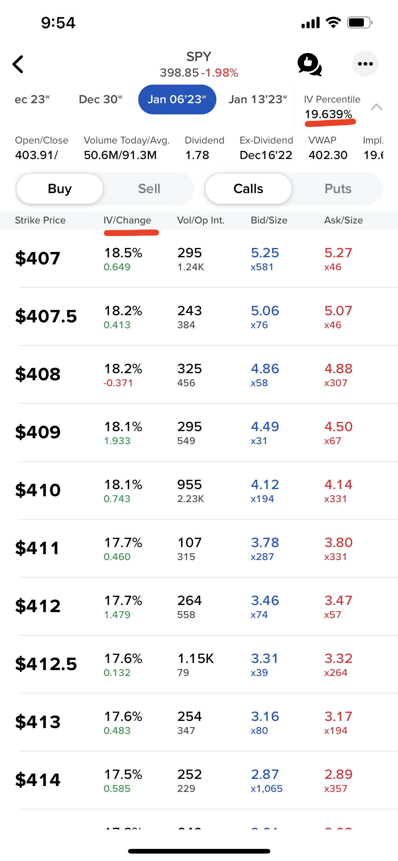
Lacking far OTM quotes for single stocks means that this is usually ruled out I would say. Either way, the VIX and a 1m ATM IV is very similar as can be seen here. How IV percentile is computed can only be guessed without a documentation. I suspect it will be simply the ATM vol for the selected expiry compared to some set number of past days. So the 19% in your example means that ~20% of days had lower, ~80% of days had higher ATM IV for that expiry in the observed time span. That it is close to current IV is a coincidence in this case, because it could be any number between 0 and 100.
Some people interpret IV as a forward looking measure of standard deviation, just like the commonly used definition of historical / realized vol which is computed as the sample standard deviation of log return as shown here. However, one should be cautious when comparing IV to historical vol (HV) - also called realized volatility (RV) - because it is not necessarily useful for at least two reasons:
1 ) Empirically, IV tends to overestimate RV, commonly referred to as Volatility Risk Premium
2 ) IV is the only free parameter in the Black-Scholes-Merton (BSM) model. Higher IV can be a result of compensation for tail risk.
A simple explanation is that market participants tend to overestimate the likelihood of a significant market crash, which results in an increased demand for options as protection against an equity portfolio. This can be exploited, as for example demonstrated in Sullivan, R., Israelov, R., Ang, I., & Tummala, H. Understanding the Volatility Risk Premium. The authors show that the returns of an investor who sells the same 5% out-of-the money put option every month, delta hedges it and holds it to expiration generated 1.5% annualized returns with a Sharpe ratio of 0.68. Compared to the S&P Sharpe Ratio of 0.32 over the same observation period (1996-2016), this is an attractive strategy.

What is IVOL?
IVOL is turning an option price into a comparable number (it’s also annualized). The theory to construct IVOL is based on the world of Black Scholes (its assumptions). Black Scholes implies normally distributed stock returns, whereas real (stock) returns are negatively skewed and have fatter tails because:
stocks (or other underlyings) tend to move down faster than they move up, so the left side has a fatter tail than the right side - known as skewness
extreme price movements in both directions (called outliers) are more common than the normal distribution suggests, so both tails are fatter than a normal distribution would suggest; known as kurtosis
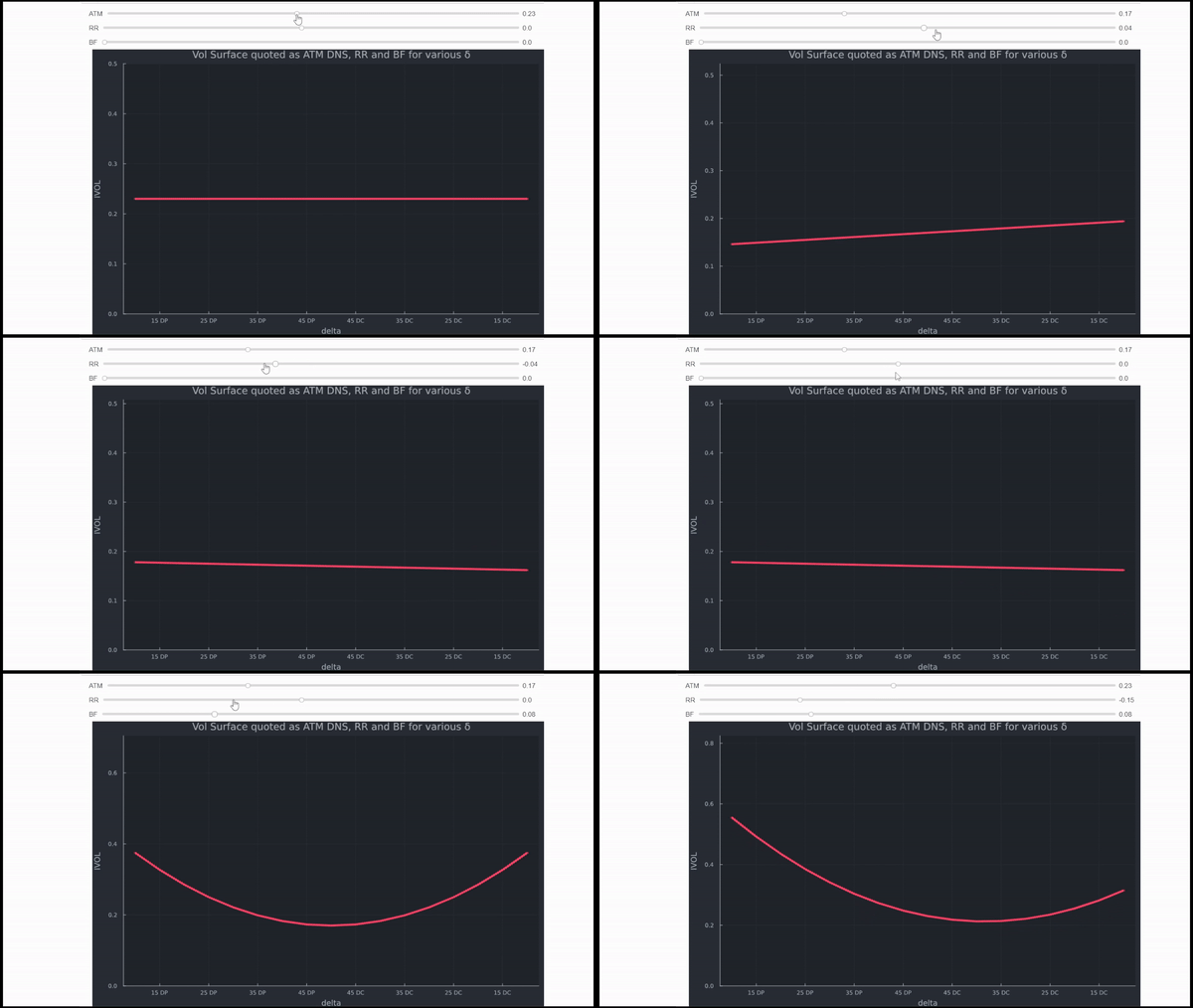
The intuition is the same for all sorts of markets. However, FX is very helpful in getting an understanding of it. Ignoring all details, FX is quoted in IVOL, the quotes come as ATM DNS (delta neutral straddle), RR (Risk Reversals) and BF (Butterflies).
In a nutshell,
- ATM determines the level (you can think of it as the Black Scholes IVOL for a specific tenor),
- RR the skew (how its tilted, towards OTM puts for RUB and GBP in the examples below) and
- BF the kurtosis (how pronounced the general wings are).

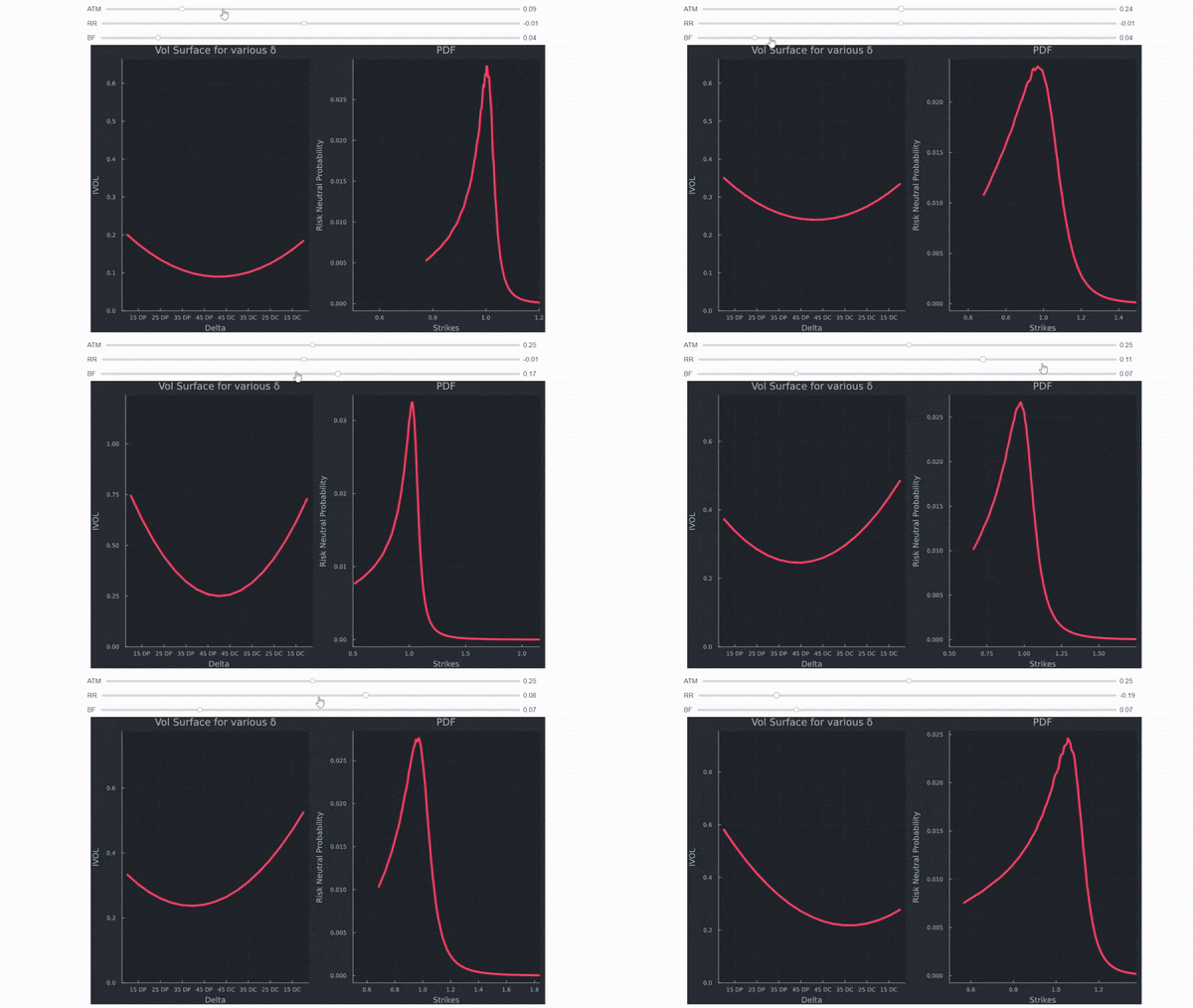
Hence, the vol surface exists mainly because there are fat tails, skewness, heteroscedasticity, jumps (crashes), and so forth. None of these real-world phenomena are featured in the Black Scholes formula. The market just developed ways to account for many of the shortcomings of Black Scholes. Using the vol quotes from above, one can compute strikes (for simplicity I assumed delta premium excluded to avoid using root solvers), back out option prices, and compute risk neutral implied probabilities for the underlying. I use the method shown by Malz in the Fed Staff Report No. 677 on June 2014 A Simple and Reliable Way to Compute Option-Based Risk-Neutral Distributions. I modified it a bit because the strikes derived from delta quotes do not lie on a uniform grid (they do not have constant spacing), in which case a more general formula for weighting is needed. All computed prices are monotonically decreasing, showing that the results are free from vertical spread arbitrage opportunities.
That way, it is easy to show how the quotes indeed affect the implied return distribution of the underlying.

A few observations:
- increasing ATM vol moves the vol surface up, and spreads out the RN probability distribution
- increasing BF quotes moves the tails out significantly
- a negative RR quote increases the left tail, a positive the right tail
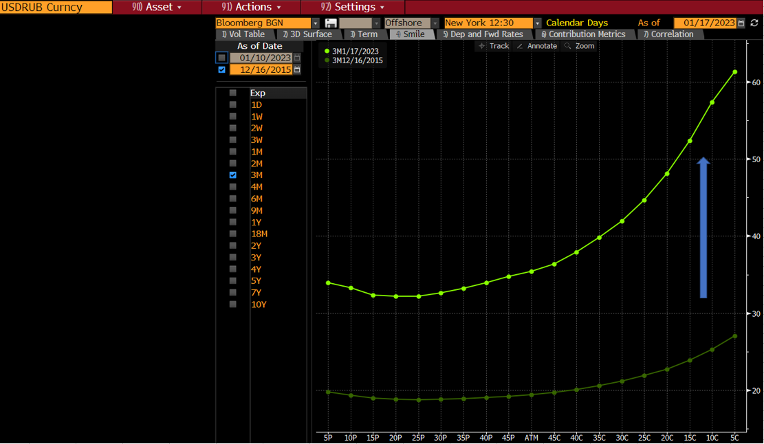
Since the Russian invasion of the Ukraine, it is more likely for the RUB to depreciate compared to the USD. If you look at a vol surface skew now, compared to a date prior to the invasion (where no one was expecting it yet), you see that the skew is a lot more pronounced now. It always existed, because the USD is generally more stable. Also, the overall level of IVOL increases too, but the main take-away is that the skew got a lot larger. To the right, we have OTM calls (on USD, which is a put on RUB, hence buying protection against a RUB depreciation is more expensive now).

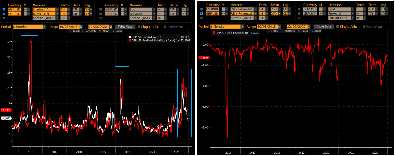
Similarly, if you look at GBP, you have Brexit as a major event. Uncertainty meant that IVOL not only anticipated the higher realized / historical vol (shown on the left screen below which is from Bloomberg's VOLC, comparing ATM 1M IVOL with realized 1M vol), but also meant that it was heavily skewed towards OTM Puts (on GBP) as displayed by the risk reversal quote over time. Realized vol takes time (1m in the example) to be computed, whereas IVOL is forward looking. That is why the spikes of the white line are before the red.

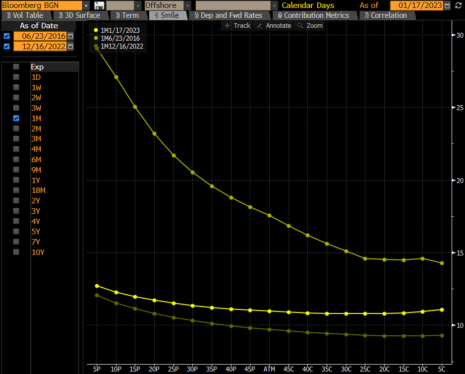
You can see that Brexit, Covid and the Russian invasion all elevated ATM IVOL (left), but the effect on the skew was a lot more pronounced during Brexit because that was a GBP specific risk. Below is a screenshot of the smile on the day of Brexit and during normal times.

Long story short, different IVOL for different strikes accounts for the possibility of larger outliers and skewness in the return distribution, thereby accounting for a short coming of the Black Scholes model.
How to compute a vol surface
With regards to your comment to @Grade 'Eh' Bacon where you wrote
you still did not answer how the total IV surface is calculated
What you look at is not a IV surface. It is simply an isolated computation for the given quoted options. You have the inputs into Black Scholes, and solve for IV, nothing more. Although doing this for an American option is not that simple after all.
If you wanted to get a vol surface, you would do something along the line of:
Filter out stale prices, unreasonable small or large bid/ask spreads, figure out a way to handle that the underlying asset and options on the asset can trade during different times on different exchanges, that there exist erratic prices, especially close to the opening and closing times of the trading session... Sorting all these difficulties out, still leaves a major problem. There is no consensus on how to model (cash) dividends, and you have borrow costs/funding costs. You can use a (continuous) dividend yield, cash dividends (implying that the observed stock price cannot follow geometric Brownian motion...), discrete proportional (discrete stock) dividends and so forth. Typically, a blend is used that uses different types for different maturities (due to lack of better data mainly).
Put another way, the problem is that the forward price is not directly quoted for listed options markets. Yet is an important quantity impacting option prices and implied volatility. Futures may be quoted but maturities frequently do not coincide with (all) option maturities. Interpolation is not trivial because future dividends (even times of payments) are usually unknown. Therefore, most practitioners (in my experience) use vanilla equity options to back out (implied) dividends. As stated in the question, the problem hereby is that put-call parity for American-Style options does not hold. Even for European-Style options, there are frequently issues with different trading times and erratic option prices etc. Since dividend payments are discrete in nature, you require a dividend schedule with dates and amounts to derive an implied dividend curve. This curve is usually noisier than one would hope for and commonly smoothed (via Kalman filter of the like).
Ignoring all these problems, de-americanization is a major building block and can be done like this:
Estimate the forward using spot, interest rates, dividends (forecasts) and ideally borrow costs/funding costs.
Use a local volatility model consistent with options of all strikes at this maturity. Alternatively, and a lot faster and simpler, compute the Black implied volatilities from put and call prices by using the estimated forward (implied forward in future iterations as explained below). This usually requires a PDE solver (or you use a binomial/ trinomial tree again). Lastly, use the estimated forward and the
implied volatilities in the Black model to compute the corresponding European option prices.
Imply the forward and dividends using the two nearest strikes on either side of the estimated forward from step 1 (make sure you quotes are reasonable for both puts and calls). The implied forward is the average of the forward obtained at each of the two strikes by applying put-call parity to the European option mid prices computed in 2), and back out a corresponding implied dividend.
Evaluate the results:
- Does the implied forward lie in between the two strikes? This is a minimum requirement.
- How different is the forward from the estimated forwarded (or implied if several steps are needed)? You will need some criteria to determine the optimal stopping.
- If the result in step 4) is not satisfying, use the current implied forward in step 2) and iterate until you are satisfied with the result.
These steps will give you Pseudo European option prices, option implied forwards and option implied dividends that are consistent with the observed American prices.
The calibration of the actual vol surface should result in the chosen (Pseudo) European option prices (only OTM, sufficiently liquid...) at any maturity to match the prices from the vol surface.
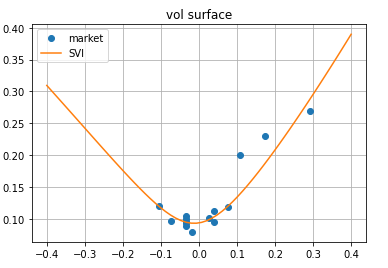
Afterwards, you will have a set of implied vols for moneyness levels, which you can fit using various techniques like SVI, SABR, or a mixture of lognormals to get a curve that best fits the existing IV and allows you to get full fledged surface for any strike and expiry.
Below is a quick SVI implementation in Python example:
spot = 1.34
forward = 1.35
t = 30 / 365.0
vols = np.array([ 12, 10, 9.5, 9, 10.5, 8, 10.24, 9.6, 11.2, 9.4, 11.9, 9.7, 20, 23,  27]) / 100
strikes = np.array([1.21, 1.3, 1.4, 1.3, 1.3, 1.32, 1.38, 1.3,
                    1.4, 1.3, 1.45, 1.25, 1.5 , 1.6,  1.8])
total_implied_variance = t * vols ** 2

def svi(k, param):
    a = param[0];
    b = param[1];
    m = param[2];
    rho = param[3];
    sigma = param[4];

    totalvariance = a + b * (rho * (k - m) + np.sqrt((k - m)** 2 + sigma**2));
    return totalvariance


def targetfunction(x):
    value=0
    for i in range(11):
        model_total_implied_variance = svi(np.log(strikes[i] / forward), x);
        value =value+(total_implied_variance[i]  - model_total_implied_variance) ** 2;
    return value**0.5

bound = [(1e-5, max(total_implied_variance)),(1e-3, 0.99),(min(strikes), max(strikes)),(-0.99, 0.99),(1e-3, 0.99)]
result = optimize.minimize(targetfunction, bound, tol=1e-8, method="BFGS")
x=result.x

K = np.linspace(-0.4, 0.4, 60)

newVols = [np.sqrt(svi(logmoneyness, x)/t) for logmoneyness in K]
plt.plot(np.log(strikes / forward), vols, marker='o', linestyle='none', label='market')
plt.plot(K, newVols, label='SVI')
plt.title("vol curve")

plt.grid()
plt.legend()
plt.show()

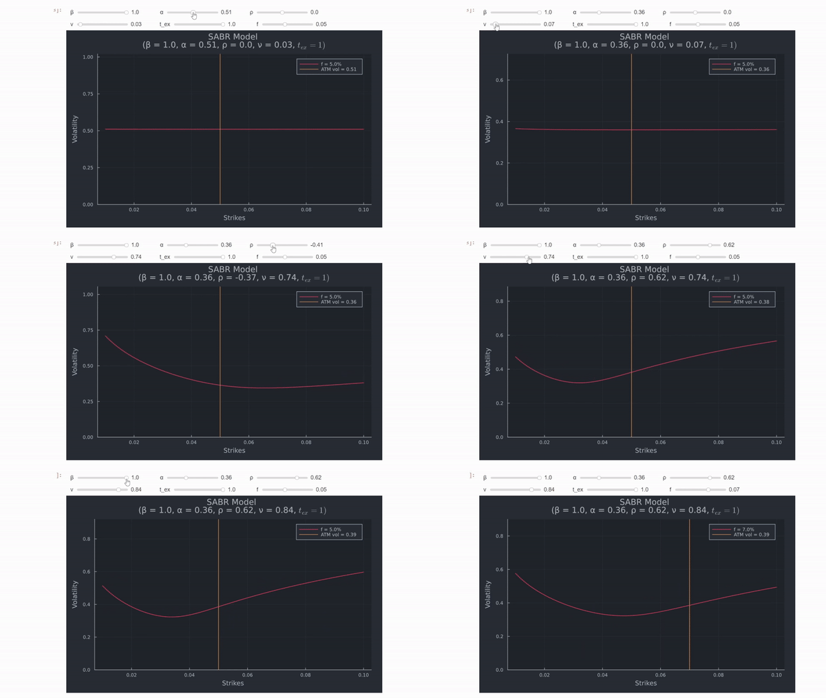
SABR calibration would involve fitting beta, alpha, rho and nu so that it resembles the shape of IV in the market. You can see details and the below illustration here.

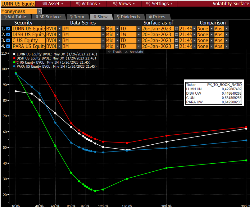
Lastly, I am not convinced about the real estate example and liquidation. Real estate is usually trading far from book value, and even the companies in the S&P500 have illiquid options markets. However, there are 14 companies in the S&P500 that trade below book value according to Bloomberg's API and the field PX_TO_BOOK_RATIO. All these have IV of deep OTM puts significantly higher than ATM, and increasing all the way.

After all, the scenario implied by such low strikes will almost surely see massive haircuts for its liquidation value as well.
