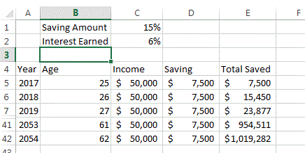
The article links to William Bernstein’s plan that he outlined for Business Insider, which says:
Put equal amounts of that 15% into just three different mutual funds:

• A U.S. total stock market index fund
• An international total stock market index fund
• A U.S. total bond market index fund

Over time, the three funds will grow at different rates, so once per year
you'll adjust their amounts so that they're again equal.

That's it.
Modelling this investment strategy
Picking three funds from Google and running some numbers.
MUTF: VTSMX  Vanguard Total Stock Market Index
MUTF: VGTSX  Vanguard Total International Stock Index Fund Investor Shares
MUTF: VBMFX  Vanguard Total Bond Market Index Fund Investor Shares
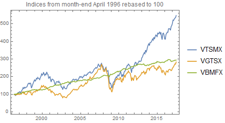
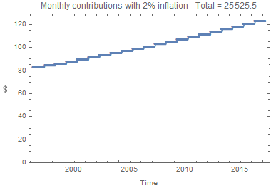
The international stock index only goes back to April 29th 1996, so a run of 21 years was modelled. Based on 15% of a salary of $550 per month with various annual raises:
annual salary   total contributions    final investment
rise (%)        over 21 years          value after 21 years
  0               20,790                    43,111
  1               23,007                    46,734
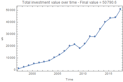
  2               25,526                    50,791
Broadly speaking, this investment doubles the value of the contributions over two decades.
Note: Rebalancing fees are not included in the simulation.
Below is the code used to run the simulation. If you have Mathematica you can try with different funds.
funds = {"VTSMX", "VGTSX", "VBMFX"};

(* Plotting the fund indices *)

{tsm, ism, tbm} = FinancialData[#, {"April 29, 1996",
     DateList[], "Month"}] & /@ funds; DateListPlot[
 Transpose[{First /@ #, 100 Last /@ #/#[[1, 2]]}] & /@
  {tsm, ism, tbm}, PlotLegends -> funds, PlotLabel ->
  "Indices from month-end April 1996 rebased to 100"]

(* Plotting the investment contributions *)

salary = 550;
investment = salary*0.15;
inflation = 2;
nmonths = Length[tsm] - 1;
ny = Quotient[nmonths, 12];
iy = Array[investment/3 (1 + inflation/100)^(# - 1) &, ny];
d = Take[Flatten[ConstantArray[#, 12] & /@ iy], 12 ny];

DateListPlot[Transpose[{Take[First /@ tsm, 12 ny], 3 d}],
 PlotLabel -> Row[{"Monthly contributions with ",
    inflation, "% inflation - Total = ",
    Total[3 d]}], PlotRange -> {Automatic, {0, Automatic}},
 PlotMarkers -> {Automatic, 6}, FrameLabel -> {"Time",
   Rotate[Style["$", 12], Pi/2]}, ImageSize -> 380]

(* Calculating & plotting the investment values *)

{tsm2, ism2, tbm2} = Take[Ratios@# - 1, 12 ny] & /@
   Map[Last, {tsm, ism, tbm}, {2}];

d2 = 0;
ds = {};
eachyear[yr_] := Last /@ Function[series,
    AppendTo[ds, Total@Array[(d[[# + 12 (yr - 1)]] +
           If[# == 1, d2/3, 0]) Apply[Times,
          1 + series[[# + 12 (yr - 1) ;; 12 yr]]] &,
       12]]] /@ {tsm2, ism2, tbm2}

vals = Array[(d2 = Total@eachyear[#]) &, ny];

rd = Last /@ Partition[Take[First /@ tsm, {2, 12 ny + 1}], 12];

DateListPlot[Transpose[MapThread[
   {{#1, #2[[1]]}, {#1, #2[[2]]}, {#1, #2[[3]]}} &,
   {rd, Partition[ds, 3]}]],
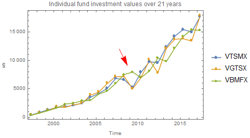
 PlotMarkers -> {Automatic, 8}, PlotLabel -> Row[{
    "Individual fund investment values over ", ny,
    " years"}], PlotLegends -> funds, Epilog -> {Red,
   Arrowheads[0.06], Arrow[{{{2007, 10, 1}, 12000},
     {{2008, 10, 1}, 9000}}]}, FrameLabel -> {"Time",
   Rotate[Style["$", 12], Pi/2]}, ImageSize -> 400]

Notice above how the bond index (VBMFX) preserves value during the 2008 crash. This illustrates the rationale for diversifying across different fund types.
DateListPlot[Transpose[{rd, vals}],
 PlotMarkers -> {Automatic, 8}, PlotLabel -> Row[{
    "Total investment value over time - Final value = ",
    Last[vals]}], FrameLabel -> {"Time",
   Rotate[Style["$", 12], Pi/2]}, ImageSize -> 400]
