With regards to a comment you made; how can you be sure you get everything else correct if your value is so wrong? With FX, there are two interest rates, IVs are usually quoted in delta (frequently Premium adjusted), and you have the issue of notional and premium currency being in different denominations (Ccy1 and Ccy2 respectively) for example.
I recommend looking at basic introductory option pricing books of the likes of
- Options, Futures and Other Derivatives, John Hull
- The Concepts and Practice of Mathematical Finance, Mark Joshi
- Paul Wilmott on Quantitative Finance, Paul Wilmott
- Arbitrage Theory in Continuous Time, Tomas Björk
- Option Volatility and Pricing, Sheldon Natenberg
For FX, I can highly recommend
- Foreign Exchange Option Pricing, Iain J. Clark
- FX Options and Smile Risk, Antonio Castagna
- FX Options and Structured Products, Uwe Wystup
In a nutshell, option pricing is entirely based on "no arbitrage" and "replication / hedging" arguments within a risk neutral framework. As a result, the derivative price does not depend on the drift / trend of the stock price. You also cannot implement the model differently because you would constantly open arbitrage opportunities.
In the simple Black Scholes world (usually called Garman Kohlhagen in FX), you still have a lot of nuances to deal with. Most FX option trading is OTC, and quotes come in IVOL directly (ATM Delta Neutral Straddles, Risk Reversals and Butterflies for several deltas). Delta itself can be premium adjusted or excluded, as well as forward or spot. In terms of quotation (EURUSD is CCY1CCY2, which means 1 EUR for how many USD), you have notional in CCY1, premium in CCY2, all else requires you to account for the change in numeraire, as shown here with code. To be precise, you also need to distinguish between price date and premium date.
How standard vanilla options are computed is shown here.
As mentioned in the other answer, in the flat vol Black-Scholes (BS) world using the usual BS notation, the fair price of the cash or nothing option is e^(−rt)*N(d2) which is the discounted probability of the option expiring in the money.
To compute this in Julia, all you need is this code:
using Distributions, Dates

N(x) = cdf(Normal(0,1),x)

# Fwd
function GKF(F,K,t_d,t_e, ccy2, σ)
    d1 = ( log(F/K) +  0.5*σ^2*t_e ) / (σ*sqrt(t_e))
    d2 = d1 - σ*sqrt(t_e)
    c  = exp(-ccy2*t_d)*(F*N(d1) - K*N(d2))
    return c, exp(-ccy2*t_d)*N(d2)
end
where t_d and t_e is time to delivery and time to expiry. The rest is standard Black Scholes logic, and I used the forward to avoid having to compute the second, less liquid interest rate, which is frequently implied from covered interest rate parity to make the model internally consistent and arbitrage free.
Using market data and converting the risk free interest rate into a continuous analog looks like this.
ccy2 = 0.0007897 # USD
σ = 6.747/100.

price_dt = Date(2020,12,30)
premium_dt = Date(2021,01,04)
expiry_dt = Date(2021,3,31)
delivery_dt = Date(2021,4,06)
days_to_expiry = (expiry_dt - price_dt)
days_to_delivery = (delivery_dt - premium_dt)

r2_cont = log(1+ccy2*days_to_delivery.value/360)/(days_to_delivery.value/365)
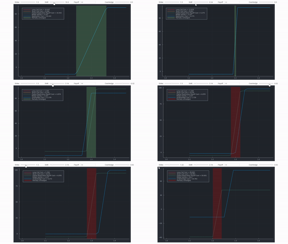
That’s it really. In real world settings, following the logic of no arbitrage and replication, market practitioners like to find ways to replicate payoffs. For example, just like Variance swaps have a theoretical replication, the payoff of digitals can be replicated with a tight call spread to capture skewness. For example, setting strikes at 𝐾± = 𝐾 ±1/2𝑑𝐾. My answer to your first question used a figure showing that an over-hedge will cost more than the centred hedge on the barrier strike, because its payoff is strictly higher. As mentioned, there are details that are omitted in this figure (the payoff diagrams would shift slightly, reflecting different costs for the premium). The gif below will show the same information but uses accurate computations that match the replication of Bloomberg below. It uses unrealistic spreads and shifts to make the distinction clear.

On the downside, this is more involved. The benefit is that it allows you to take into account the IV skew. Generally, the price difference will be marginal and it is safe to avoid this. It will also be hard to implement because it involves fitting a vol surface. If you try to do it, these are the steps:
Compute the spread
function spread(K,shift)
      lower_K = K*(1-shift/2)
      upper_K = K*(1+shift/2)
      spread  = upper_K-lower_K
      return lower_K, upper_K, spread
  end

      strike = 1.22
  spr = spread(strike,0.01)
  val = ("Lower","Upper","Spread")
  k = Dict(zip(val,spr))
Compute the needed notional adjustment because the spread will payoff the difference between the lower and higher strike only. The spread between strikes * Notional is the sum of the payoffs.
 function notional_adj(N,spread,payoff)
      return payoff/(spread*N) end
Get fitted vols for the spread from the vol surface (usually pulled via a logic as shown here for example). I used Bloomberg's API to fetch the IV needed for the spread. The pricer itself (OVML) only displays the vanilla vol.
σ = Dict("Mid" => 6.747/100, "Lower" => 6.78047/100, "Upper" => 6.73819/100)
Fetch the results and compare to Bloomberg:

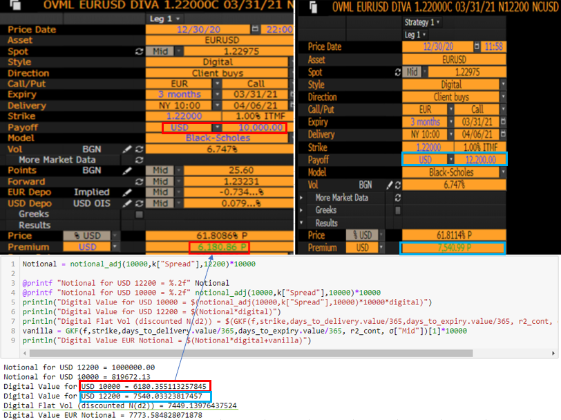
You can see that the Notional needed was already ~ 819.6K and 1M for such small cash or nothing digitals and a 1% spread. It does not match BBG perfectly, but the difference is less than 1 USD. Moreover, the difference to the flat vol Black-Scholes (BS) world is only ~ 90 Euros.
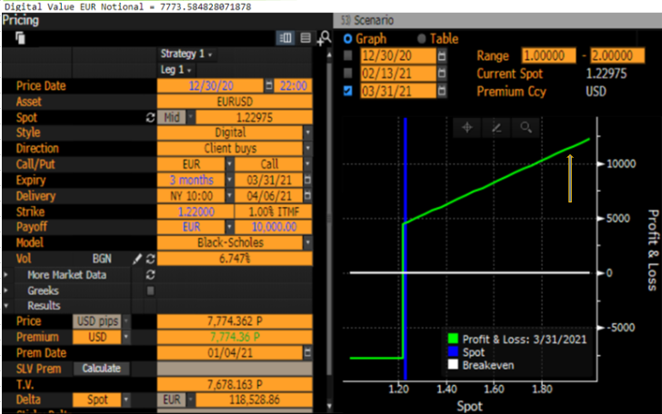
In the EUR notional case, you have another issue, namely that it is no longer a cash or nothing, but an asset or nothing binary option. The final exchange rate will matter for your actual payoff in this case which is why it is scaled by a vanilla call option and the BBG screenshot below shows an upward slope in the scenario tab above strike.
