Option Theta: What conditions are needed for Theta > P/N, where P = option price, and N = days to expiration?

Question

The wikipedia definition for Theta is:

And people frequently refer to the picture below, to show what typically happens with an option's value as a function of time; we can note this is non-linear, with the highest time loss occurring as one gets close to expiration. As such, generally speaking, one (I) would expect that at any given point in time, the theta of an option would generally be less than its current price, divided by the days remaining; the reason being, it's going to continue to decay faster, in a non-linear manner.

So, if an out-of-the-money option (all time value) has a price P (say $3.00), and there are N days to expiration (say 45), can you help me understand scenarios where theta would be 1) greater than P/N ( > $3.00/45) and 2) less than P/N?

Final Note: From the recent far out-of-the-money PUT options I looked at on SPY, in each case they fell into case 1 to my surprise. With 45 days to to expiration, their theta was significantly higher than their price divided by 45. So, I'm wondering what conditions result in case 1 -- what causes this to happen?

Answer 1

So, if an out-of-the-money option (all time value) has a price P (say $3.00), and there are N days...

The extrinsic value isn't solely determined by time value as your quote suggests. It's also based on volatility and demand. Here is a quote distinguishing between extrinsic time value and intrinsic non-time value:

The time value of an option is entirely predictable. Time value premium declines at an accelerating rate, with most time decay occurring in the last one to two months before expiration. This occurs on a predictable curve.

Intrinsic value is also predictable and easily followed. It is worth one point for every point the option is in the money. For example, a call with a strike of 30 has three points of intrinsic value when the current value of the underlying stock is $33 per share; and a 40 put has two points of intrinsic value when the underlying stock is worth $38.

The third type of premium, extrinsic value, increases or decreases when the underlying stock changes and when the distance between current value of stock and strike of the option get closer together. As a symptom of volatility, extrinsic value may be greater for highly volatile underlying stock, and lower for less volatile stocks. Extrinsic value is the only classification of option premium that is unpredictable.

The SPYs you point out probably had a volatility component affecting value. This portion is a factor of expectations or uncertainty. So an event is expected to conclude prior to expiration, but an unknown outcome can cause theta to be higher than p/n. For example, a drug company is being sued and the outcome of a trial will determine whether that company pays out millions or not. The extrinsic will be higher than p/n prior to the outcome of the trial then drops after.

Of course, the most common situation where this happens is earnings. After the announcement, it's not unusual to see a dramatic drop in the extrinsic portion of options. This is why sometimes a new option trader gets angry when buying calls prior to earnings. When 'surprise' good earnings are announced as hoped, the rise in stock price is largely offset by a fall in extrinsic value giving call holders little or no gain!

As for the reverse situation where would theta be lower than p/n would expect? Well you can actually have negative theta meaning the extrinsic portion rises over time (this statement is a little confusing because theta is usually described as negative, but since you describe it as a positive number, negative here means the opposite of what you'd expect).

This is a quote from Option Volatility & Pricing¹. Keep in mind that they use 'positive' theta to mean the time value increases up over time:

Is it ever possible for an option to have a positive theta such that if nothing changes the option will be worth more tomorrow than it is today? When futures options are subject to stock-type settlement, as they currently are in the United States, the carrying cost on a deeply in-the-money option, either a call or a put, can, under some circumstances, be greater than the volatility component. If this happens, and the option is European (no early exercise permitted), it will have a theoretical value less than parity (less than intrinsic value). As expiration approaches, the value of the option will slowly rise to parity. Hence, the option will have a positive theta.

---

¹ Sheldon Natenberg. Option Volatility & Pricing: Advanced Trading Strategies and Techniques (Kindle Locations 1521-1525). Kindle Edition.

Answer 2

The chart in the question applies to near-the-money options and is misleading for sufficiently out-of-the-money options. For at-the-money, the option price is proportional to the expected absolute move over the remaining life, i.e., $\sigma \sqrt{N}$ where $N = T - t$. This shape (sideways parabola) is what the chart shows.

However, far out-of-the-money, the option price $P$ is mainly affected by the probability of reaching the strike: $P \sim \Delta \sim \exp(-\frac{z^2}{\sigma^2 N})$. This is the dominant factor in the Black-Scholes formula. Here $z$ is the move the underlying needs to make to reach the strike. The ratio $\Theta/P$ (fractional decay rate) is then roughly $\frac{z^2}{\sigma^2 N^2}$. So $\Theta$ is greater than $P/N$ if $\frac{z^2}{\sigma^2 N}$ is sufficiently large, i.e., if $\Delta$ is sufficiently small.

The option can decay so rapidly that it loses most of its remaining value each day, even if it has weeks left, due to the sensitivity of the exponential. The fractional decay accelerates, even though the dollar decay ($\Theta$) does not.

The answer by derivs is qualitatively correct, that far out-of-the-money options decay to effectively zero well before expiration.

Answer 3

The OP is no longer active, but a lot of people looked at this question, which is based on a misunderstanding of what theta is. If you type the formula in Wikipedia into excel, you should see that it matches your data provider. Technically, SPY options are American, but given the option at hand, there is no difference to a European option anyways. In general, the difference, especially in theta will be very small.

Most users here will not see closed questions on quant.stackexchange, but if you do, you can look here. The screenshot with the values looks like this:

Instead of Excel, I will use Julia because charting will be easier and interactive. In any case, you can almost copy paste the code for the Greeks and option value from the wikipedia link provided in the question. As mentioned there, theta is expressed in value per year and usually divided by the number of days in a year.

using Interact,Plots, Distributions,DataTheta Frames, PlotThemes, Dates, PrettyTables, Interact

N(x) = cdf(Normal(0,1),x)
n(x) = pdf(Normal(0,1),x)

"""
Calculate Black-Scholes European call option price
https://en.wikipedia.org/wiki/Greeks_(finance)#Formulas_for_European_option_Greeks
"""
function OptionBlackSPs(S,K,t,r,d,σ)
  d1 = ( log(S/K) + (r - d + 1/2*σ^2)*t ) / (σ*sqrt(t))
  d2 = d1 - σ*sqrt(t)
  p = -exp(-d*t)S*N(-d1) + exp(-r*t)*K*N(-d2)
  delta_p = -exp(-d*t)*N(-d1)
  gamma_p = exp(-d*t)*n(d1) / (S*σ *sqrt(t))
  theta_p = (-(S * exp(-d*t)*n(d1)* σ )/ (2 * sqrt(t)) + r * K * exp(-r*t) * N(-d2) - d * S * exp(-d*t)*N(-d1))/365
  rho_p = -( K*t * exp(-d*t) * N(-d2))*0.01
  vega_p = S * exp(-d*t)*n(d1) * sqrt(t)*0.01
  return delta_p, gamma_p, theta_p, vega_p, rho_p, p
end
df= DataFrame("Days"=> reverse(days), "Delta" => [x[1] for x in res], "Gamma" => [x[2] for x in res], "Theta" => [x[3] for x in res], "Vega" => [x[4] for x in res], "Rho" => [x[5] for x in res], "Theoretical value" => [x[6] for x in res], "Theta Bumped" => theta_bump, "P/N" => p_n)

hl_1 = Highlighter((data,i,j) -> data[i,1] == 42, crayon"bg:dark_gray white bold")
PrettyTables.pretty_table(df,  border_crayon = Crayons.crayon"blue", header_crayon = Crayons.crayon"bold green", formatters = ft_printf("%.4f", [2,3,4,5,6]), highlighters = (hl_1))

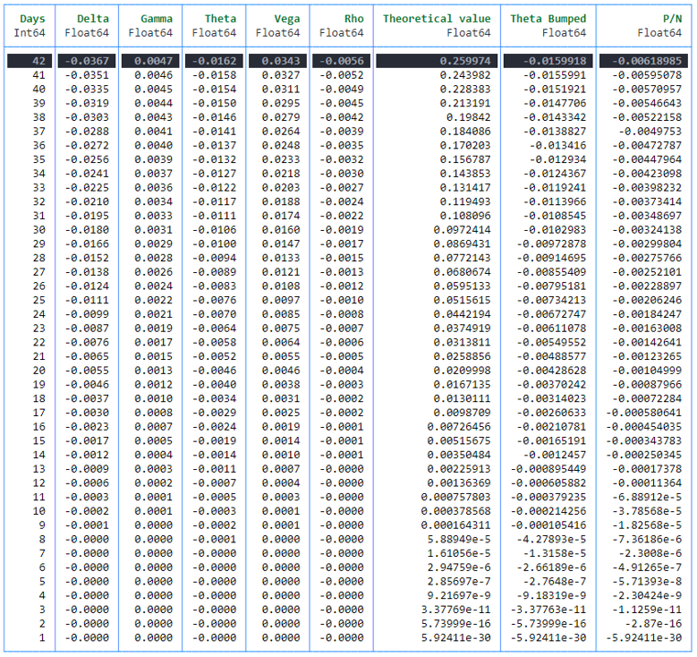
The dataframe below is the result, with the first line being the option priced in the screenshot above. As you can see, it unsurprisingly (it is just Black Scholes) matches exactly.

The other lines shorten time to expiry by one day at a time, keeping all else equal. Theta bumped is the finite difference computation of theta (shorten by one day, look at the difference as shown here. You simply cannot multiply theta by the number of days because theta changes with time (t is part of the formula).

With regards to P/N, that also does not work because theta shows the change in price for one day, not some average per day, spread equally over the options life.

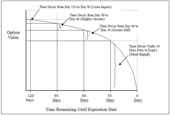
The problem with the chart, and the interpretation that

one would expect that at any given point in time, the theta of an option would generally be less than its current price, divided by the days remaining; the reason being, it's going to continue to decay faster

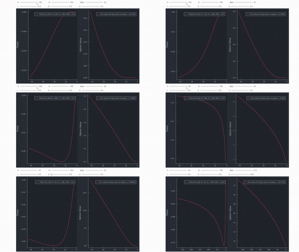
is that looking blindly at a single figure tells you little about option pricing. If you think a bit about the figure, you will quickly realize that it can only be for an ATM option because an ITM option will not be worth zero at expiration, and an OTM option will already be worthless some time prior to expiry. Therefore, there will be an inflection point somewhere after which theta goes towards zero (as in the dataframe above). Since we already have a completely dataframe, we can make an interactive chart using a syntax similar to the one used here.

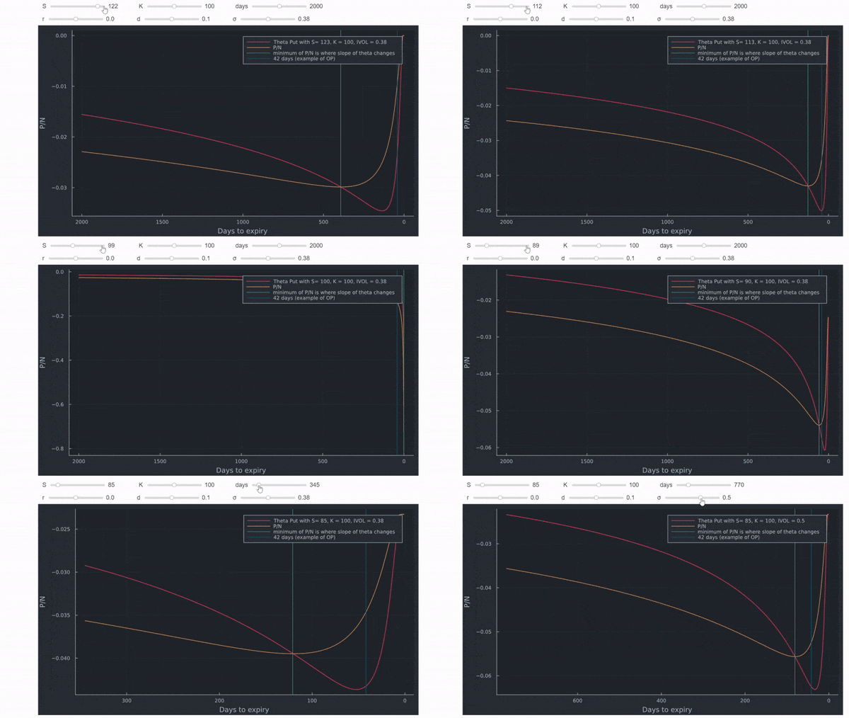
So is there any relation to P/N at all? Yes! Theta crosses P/N from above at the lowest level of P/N when plotted with time remaining until expiration. This point corresponds graphically to the falling inflection point of theta. Where this occurs depends a lot on moneyness and IV, similar to any other value in option pricing. The vertical blue line is the 42 days of the option in the example of the OP.

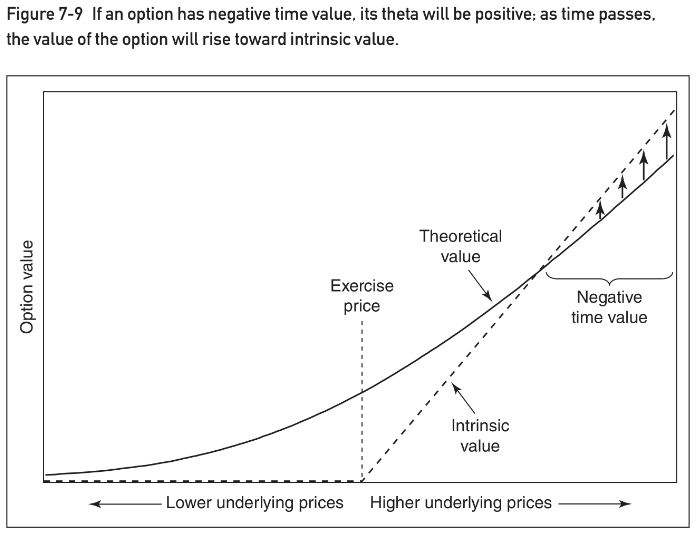
The Natenberg example mentioned in another answer is from futures, which does not apply to ETFs (SPY). Natenberg however has a similar argument for stock options on P. 109 which goes like this

Is it ever possible for an option to have a positive theta such that if nothing changes, the option will be worth more tomorrow than it is today? In fact, this can happen because of the depressing effect of interest rates. Consider a 60 call on an underlying contract that is currently trading at 100. How much might this call be worth if we know that at expiration the underlying contract will still be at 100? At expiration, the option will be worth 40, its intrinsic value. However, if the option is subject to stock-type settlement, today it will only be worth the present value of 40, perhaps 39. If the underlying price remains at 100, as time passes, the value of the option must rise from 39 (its value today) to 40 (its intrinsic value at expiration). The option in effect has negative time value and therefore a positive theta. It will be worth slightly more as each day passes. This is shown in Figure 7-9.

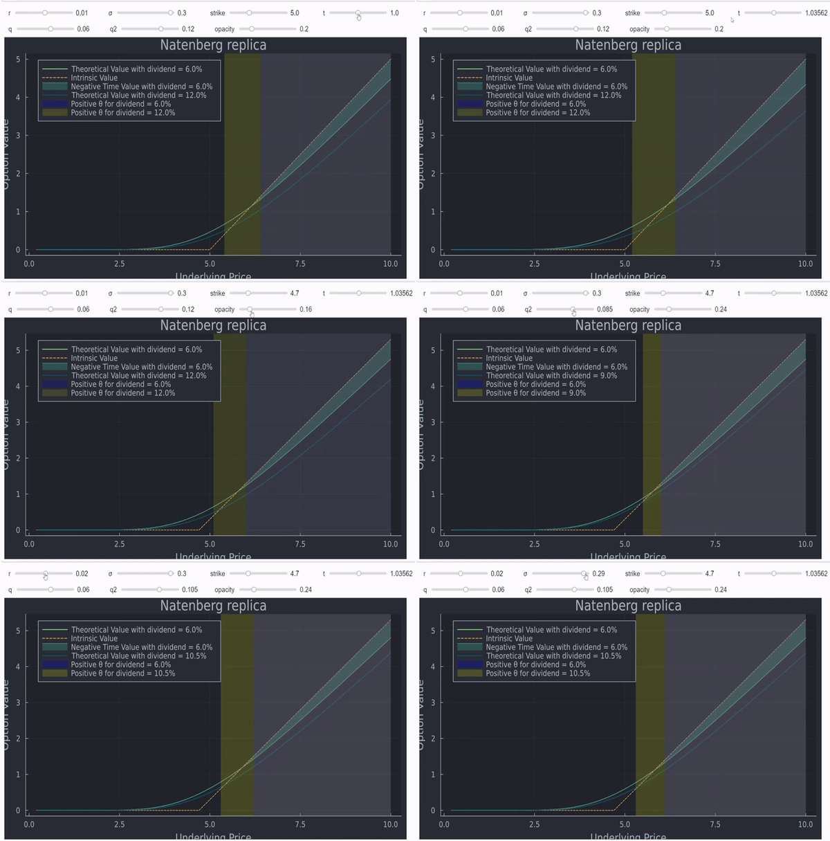
I replicated this in code here.

• the shaded area in the curve in green shows where there is negative time value for the option with dividend set to q (9% in this example)
• the blue curve is the payoff for the same option but with dividends set to 12%
• the shaded bars show the areas where Black Scholes theta is positive (blue for q = 9% and yellow for q2 = 12%) - note that the blue bar overlays parts of the yellow bar

• It closely resembles the chart from Natenberg, and given the impact of r and q on the option (and forward), this shape makes intuitive sense
• Theta itself is also closely related to that area as is visible by the coloured bars starting more or less at the intersection of the option value with the intrinsic value

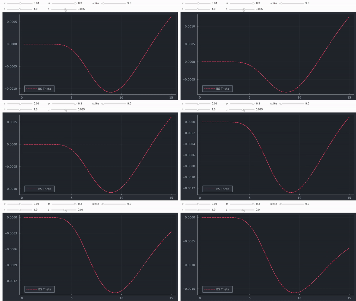
It is not a formal prove but in my opinion, often intuition and charts are also very useful. Last but not least, one can also plot theta as a function of spot to see that it indeed turns positive for (deep) ITM options with positive dividends:

That also shows that Natenberg's explanation is incorrect - and it is dividends, not the depressing effect of interest rates that is at work here.

With regards to the answer provided by @nanoman, the same applies for ITM options as shown in my gifs (you need to exclude intrinsic value because it is not affected by time or IV).

Answer 4

Excellent question. Easy answer.

You are looking at out of the money options, and my guess is they are quite out of the money. I am not the best writer so let me try to explain by way of an example.

Assume an at the money call option (100 strike) is worth $3.00

Assume the 120 strike is worth $1.00

Assume the 140 strike is worth $.20

Assume the 150 strike is worth $.00

We see that way prior to expiration, the 150 strike is already worth zero. It is therefore fair to assume the 140 strike will be worth zero shortly, way prior to expiration. For purposes of the example, let's assume it will be zero in seven days. Therefore all its decay will occur over the next seven days and as the above example is 45 days, 38 of those days will have a theta of 0.

This is why you are seeing what you are. You are assuming zero in 45 days when the life of the extrinsic value is only 7 days.

As you move closer to the at the money options you will see the p/n ratio performing more as you expect, and when you arrive at the at the money options, it is impossible for theta to be more than extrinsic divided by days as the sum cannot be worth more than the parts.

Hope that made sense.

In addition, every reply about events and earnings being the cause is wrong. A standard option model just does not assume that volatility will change from its current input, it is not that sophisticated. I have written ones that do that, but for much more complicated purposes than standard options.

Also, whoever wrote the information from tradingmarkets.com (inserted in the reply by robotcookies) knows nothing about options and I would avoid that author like the plague.

-Regards